Introduction

Scaling is a crucial pre-processing step for many High-Dimensional data analysis algorithms. For those algorithms, data should be properly scaled to generate reliable results.

Among the many types of scales available in FCS Express, Biexponential scale is of particular interest since it is the only one able to automatically detect the transition point (i.e. Below Zero parameterreferred to as BZ henceforth) based on the data. This is a great advantage in Flow Cytometry, since different parameters might require a different BZ (due to differences in data distribution between them).

The automatic detection of the BZ is robust and there is a very good chance that good setting is found for each parameter, without the user’s manual intervention. However, in the presence of outliers in the negative range, the automatic BZ calculation might be biased, resulting in very high BZ values.  Graphically this is recognizable by a distorted negative population and by an increase of the extent of negativity for the parameter range.

In the example below, the cFluor V420-A parameter has been scaled using the Biexponential scale with automatic BZ detection. In the first two samples, the data are properly scaled without manual intervention (BZ has been automatically set to ~4312 and ~4643 respectively). However, the huge presence of outliers in the negative range in the third sample, led to a BZ value of 1.4x10⁶. The scaled data of each sample are depicted in the histograms below.

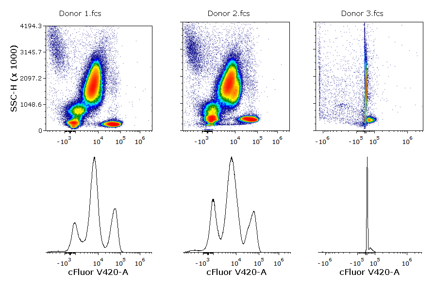
In flow cytometry, the classical manual data analysis expects the user to open 1D and/or 2D plots and visually inspect them. For this reason, it is easy to spot scaling issues like the one above.

With High-Dimensional data analysis, it is a misconception that visual inspection is only required to review the final result. This is risky, as every intermediate step in an High-Dimensional data analysis pipeline generates results that should be quality controlled, including Scaling.

When Scaling is used in a High-Dimensional data analysis pipeline, is a good practice to check the result of this transformation to ensure that the scale applied is appropriate. This is true regardless of the type of scale, but especially true when the Biexponential scale is used in conjunction with automatic BZ detection as outliers in the negative range might bias the calculation.

Real-data Example

In the example below:

• The three samples used in Figure 1 have been concatenated (merged) to perform High-Dimensional data analysis.
• A data cleaning algorithm that requires a Scaling step (i.e. FlowCut) is run on the ungated population.
• The scaling is run independently on each sample (this is done by leveraging the Classifications Folder pipeline step).
• The Biexponential scale is used and is set to automatically calculate the BZ.

As mentioned above, this is a specific scenario but it’s worth addressing, since none of the four conditions above is per se rare:

• Data Merging is very often used in High-Dimensional data analysis.
• Applying a scale on the ungated population might be needed to pre-process data for specific algorithms (e.g. FlowCut, which is used in this example, requires data scaling and, since it is a data cleaning algorithm, it is usually run at the very beginning of the analysis on ungated data).
• A Classification Folder is used every time an algorithm should be run independently on each sample in a merged file (e.g. cleaning algorithms are good examples).
• The automatic detection of the BZ is used very frequently (probably most of the time when using Biexponential scale) given its advantages.

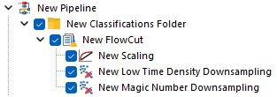
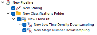
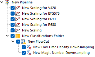
This is how the pipeline described above would look in FCS Express. Note that, since FlowCut is created within the Classification Folder, the Scaling step is also within that folder.

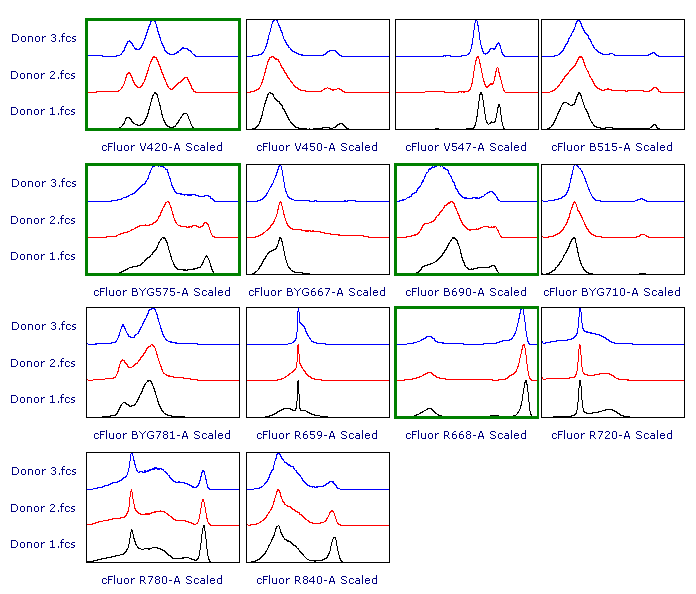
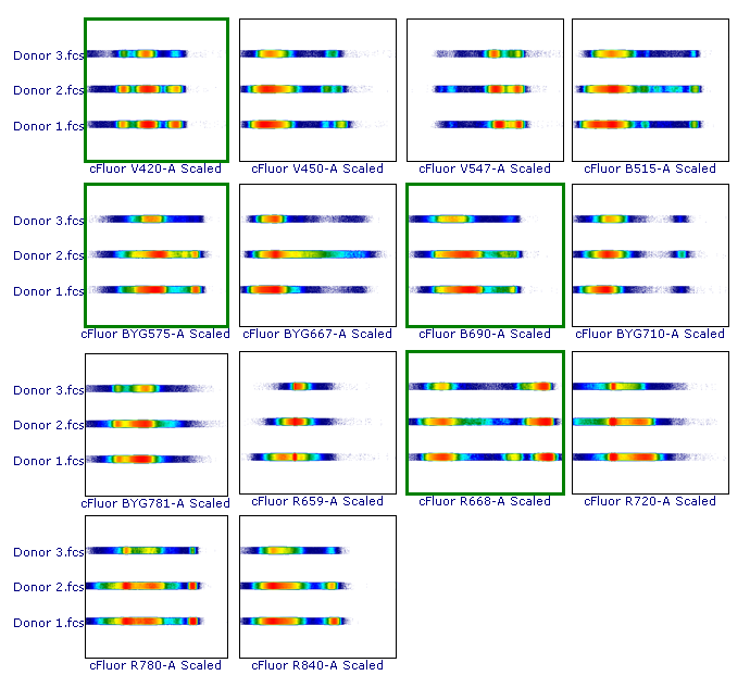
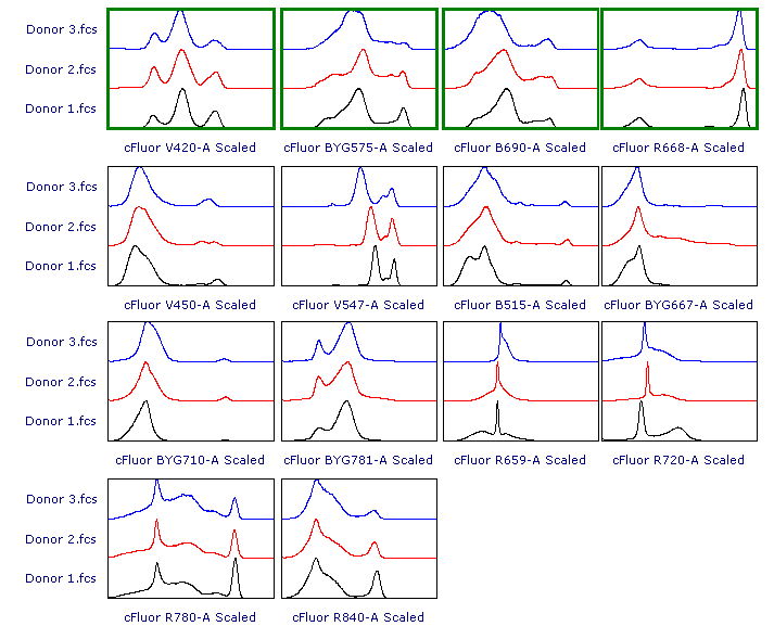
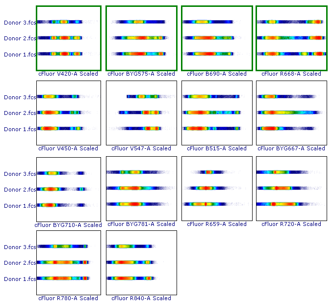
As suggested, let’s review the results to check whether each of the samples has been properly scaled. This can be done using either 1D histograms (top pane) or 2D plots (bottom pane).

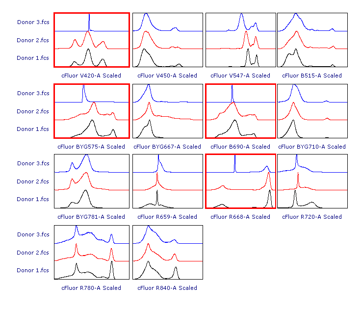
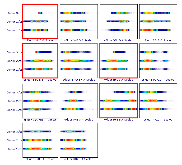
As you can see, File 3 displays aberrant scaling for some parameters (red frames). This is caused by the presence of outliers in the negative range (similar to what was shown in Figure 1), which led to an overestimation of the Below Zero parameter (see the Introduction section above).

Possible Approaches

There are two possible solutions to address this issue:

1. Run the Scaling step on the whole dataset (i.e. the merged or concatenated file) instead of on each sample independently. The basis of this approach is that the outliers responsible for skewing the BZ, will be diluted enough to no longer cause this issue. This can be easily done by moving the Scaling step upstream and outside the Classification Folder. Of course, if the outliers in the negative range make up a large portion of the merged file, they won’t be diluted enough and will still bias the automatic calculation of the BZ parameter. If this is the case, this strategy won’t solve the issue.
2. Define the BZ manually for those parameters which are not properly scaled using the automatic BZ detection. This can be done by adding additional Scaling steps in the pipeline, one for each parameter that requires manual scaling. Those additional steps can be either inside or outside the Classifications folder. This approach is effective but more laborious because a Scaling step has to be created for each parameter (unless of course multiple parameters are properly scaled using the same BZ parameter; in that case they can be scaled within the same Scaling step).

Below is how the pipeline would look when strategy #1 is put in place.

Here is the result using the same data set as shown in the earlier example.

Alternatively, below is how the pipeline would look when strategy #2 is put in place.

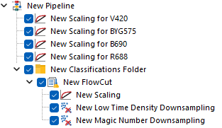
Each of the Scaling steps at the top of the pipeline, is set to scale a single parameter using a manually defined BZ parameter.

The last Scaling step is set to scale all the remaining parameters, still using Biexponential scale with automatic BZ detection. Note that this last Scaling step can either be kept within the Classification Folder (Figure 6; top pane) or upstream of it (Figure 6; bottom pane), depending on whether the automatic BZ detection is intended to be calculated file-by-file, or on the whole merged dataset respectively.

Note that strategy #2 changes the order of the resulting Scaled parameters.

Here is the result.

In this example data, the result of either strategy #1 and strategy #2 yields scaling of Donor 3.fcs that is more appropriate than the original result of Biexponential scale with automatic BZ detection.